Municipalities
Each municipality (gemeente) is represented as a single junction point with positive demand, abstracting the entire secondary and tertiary distribution network within that jurisdiction. This node serves as the sole supply point for all water within the municipality’s boundaries, with characteristics such as population, land area, and housing stock consolidated at this level.
The system presents two main challenges. First, municipal parameters evolve over time as cities grow and change. Second, the network topology itself is dynamic: municipalities can merge or be absorbed by larger neighbors, causing the number of nodes to vary throughout the planning horizon.
Excursus on the Modelling Approach
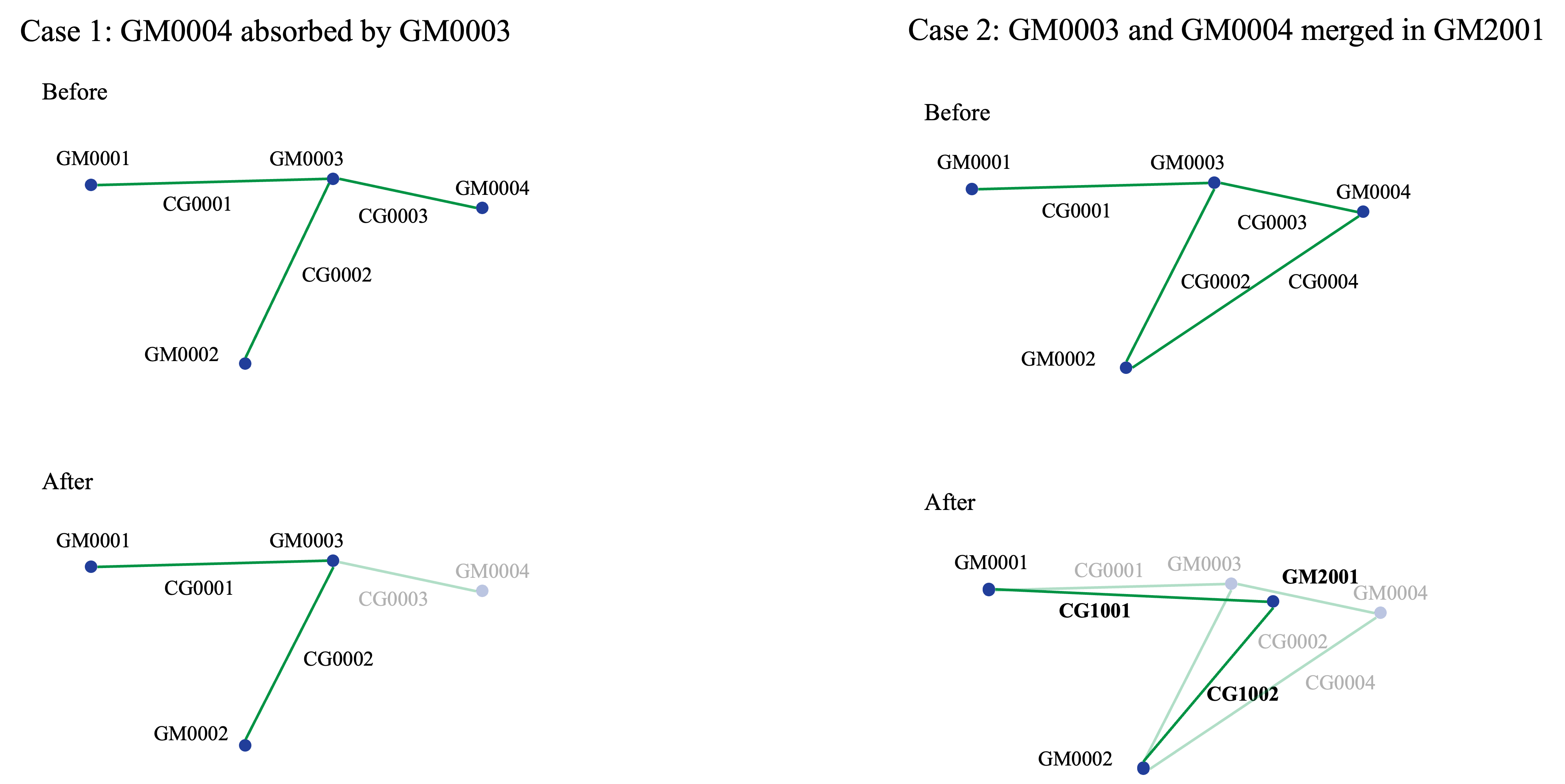
To model this administrative restructuring, municipalities can only open or close on January 1st of each year. When a municipality closes, its delivery point disappears from the network and its assets (population, land area, housing stock, etc.) are redistributed between the “destination municipalities”, with the “main destination municipality” inheriting also the hydraulic connections to other municipalities and water sources. Extensive properties (e.g., population, number of houses) are accumulated, while intensive properties (e.g., average age of the inner distribution network) are distributed using a weighted mean. Besides renaming, fig. 1 illustrates the two possible cases for dissolved municipalities1, which are:
Absorption by existing municipalities: When a municipality is absorbed by a larger neighbor that already exists, all attributes of the closing municipality transfer to the destination municipality. Any pipe that previously connected these two entities becomes hidden, as it formally becomes part of the destination municipality’s internal distribution network2.
Clustering into new municipalities: When multiple municipalities close and cluster together to form a new entity, all their delivery points disappear and a new supply point emerges at the location of the newly formed municipality. Of course, the new municipality attributes are computed by aggregating those of its constituent municipalities. Internal connections between merging municipalities become hidden as for the “Absorption by existing municipalities” case. External connections to neighbour municipalities are replaced by new connections routed to the new city centre. While it’s not possible to operate on the original connections anymore, the old connection remains active as a fallback to preserve network connectivity.
This modelling approach mirrors real-world dynamics in densely populated countries like the Netherlands. For example, when a new municipality forms through clustering, typically a new city center is established while former city centers become secondary neighborhoods. These moments of urban reorganization present natural opportunities for water utilities to lay new connections and redesign substantial portions of the distribution system.
Municipalities have many attributes that influence the other modules of the system. The full list can be seen in tbl. 1, while the actual values for these variables can be inspected within the data files, which are mapped in Appendix A.
| Property | Type | Scope | Unit |
|---|---|---|---|
| Name | Static | Municipality | |
| Identifier | Static | Municipality | |
| Latitude | Static | Municipality | degrees |
| Longitude | Static | Municipality | degrees |
| Elevation | Static | Municipality | m |
| Province | Static | Municipality | |
| Begin date | Static | Municipality | date |
| End date | Static [Optional] | Municipality | date |
| End reason and destination | Static [Optional] | Municipality | |
| Population | Dynamic Exogenous | Municipality | inhabitants |
| Surface land | Dynamic Exogenous | Municipality | \(km^2\) |
| Surface water (inland) | Dynamic Exogenous | Municipality | \(km^2\) |
| Surface water (open water) | Dynamic Exogenous | Municipality | \(km^2\) |
| Number of houses | Dynamic Exogenous | Municipality | units |
| Number of businesses | Dynamic Exogenous | Municipality | units |
| Average Disposable Income | Dynamic Exogenous | Municipality | \(k\text{€}\) |
| Average age distribution network | Dynamic Endogenous | Municipality | years |
The total municipality water demand comprises two volumetric quantities:
- Billable water demand (\(D^\text{BIL}\)): The sum of household and business water demands described in sec. 0.0.1.1.
- Non-revenue water (\(D^\text{NRW}\)): accounting for leaks, flushing, measurement errors and other losses described in sec. 0.0.1.2.
While these quantities represent the physical components of demand, they are not directly observable by participants. Instead, participants observe the total water demand divided into two components: consumption (\(Q\); delivered outflow) and undelivered demand (\(U\)).
For each municipality \(m\) at time \(t\), these quantities maintain the following relationships:
\[ \begin{aligned} D_m(t) &= D^\text{BIL}_m(t) + D^\text{NRW}_m(t) \\ &= Q_m(t) + U_m(t) \end{aligned} \qquad{(1)}\]
The decomposition between delivered and undelivered demand is extracted from an EPANET simulation of the network run in pressure-driven analysis (PDA) mode with a minimum pressure threshold of 30 m. Whenever there is undelivered demand, we assume that this reduces the billable component first, i.e., \(Q^\text{BIL}_m(t) = D^\text{BIL}_m(t) - U_m(t)\).
Water Demand Model
The methodology developed to generate water consumption time series builds on historical data from the Dutch association of water companies (Vewin, 2025), which provide nationwide trends in total drinking water production, sectoral water use, and non-revenue water over the period 2000–2024. Specifically, water-consumption time series generation is structured into three phases.
Phase I. The first phase estimates the annual water volume supplied to each municipality using information on households and businesses (CBS, 2025), complemented by projected data where required. These annual volumes are calibrated to match national totals reported in official statistics (Vewin, 2025) and then randomized around the calibrated value to introduce variability among municipalities.
Phase II. In the second phase, representative hourly consumption profiles are assigned to each municipality using a library of year-long, normalized profiles derived from district-metered areas and pre-processed to remove leakage effects. In greater detail, for each municipality, two residential profiles are selected from the library according to municipality population class, while a single non-residential profile is drawn from a dedicated set.
Phase III. The third phase produces the final hourly time series by applying a Fourier series-based approach which combines seasonal modulation, climate-related adjustments (accounting for the maximum yearly temperature), and random perturbations to capture temporal variability. The two residential profiles associated with each municipality are aggregated through weighted combinations (with the weights being uncertain), and both residential and non-residential profiles are scaled to match the previously estimated yearly volumes.
Therefore, the total billable demand of municipality \(m\) at time \(t\) (within year \(y\)) is defined as:
\[ D^\text{BIL}_m(t) = D^\text{R1}_m(t, T_y) \cdot w_m + D^\text{R2}_m(t, T_y) \cdot (1-w_m) + D^\text{C}_m(t, T_y) \qquad{(2)}\]
where \(D^\text{R1}_m(t, T_y)\) and \(D^\text{R2}_m(t, T_y)\) represent the two residential demands, \(w_m \in [0,1]\) is the unitary weight to combine them, \(D^\text{C}_m(t, T_y)\) is the (commercial) non-residential demand, and \(T_y\) is the maximum temperature recorded in year \(y\).
| Property | Type | Scope | Unit |
|---|---|---|---|
| Population | Dynamic Exogenous | Municipality | inhabitants |
| Number of houses | Dynamic Exogenous | Municipality | units |
| Number of businesses | Dynamic Exogenous | Municipality | units |
| Daily per household demand | Dynamic Exogenous | Municipality | m³/house/hour |
| Daily per business demand | Dynamic Exogenous | Municipality | m³/business/hour |
| Max yearly temperature | Dynamic Exogenous | National | °C |
Non-Revenue Water Model
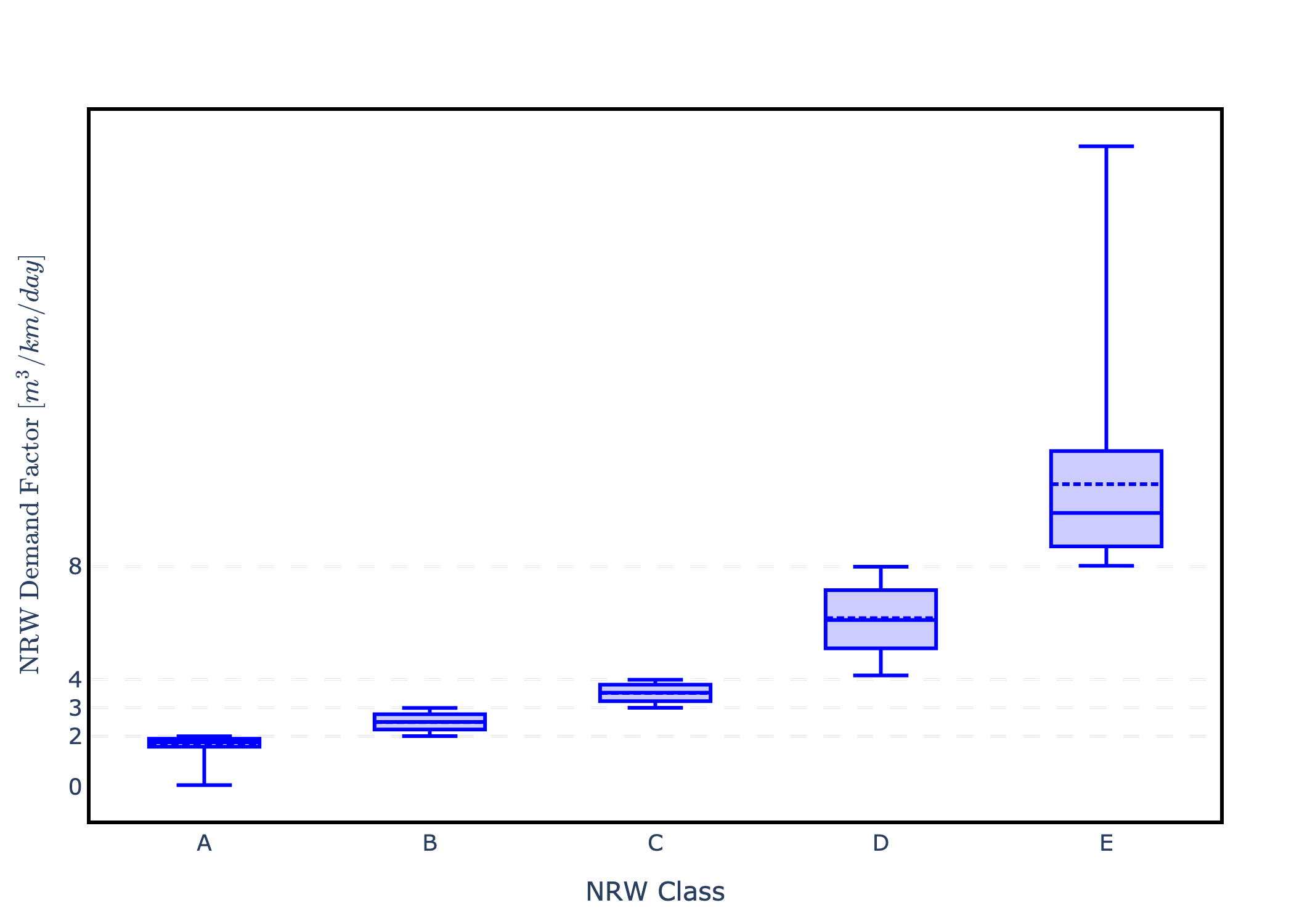
Non-revenue water (NRW) is an uncertain quantity modeled through the average age of pipe infrastructure in each municipality’s inner distribution network (IDN). Based on this average age, municipalities are assigned to one of five NRW classes as reported in tbl. 3. Each class is associated with a distinct probability distribution of NRW demands, from which daily samples are drawn to generate the volumetric NRW demand factor (\(m^3/km/day\)). Notably, older infrastructure suffers from more leaks and therefore exhibits higher NRW demand factors.
The distribution of NRW demands varies by class and is illustrated in fig. 2. The actual values of the distributions’ parameters can be inspected within the data files, which are mapped in Appendix A.
The total length of pipes in a municipality is linked to its population size through the following linear relationship:
\[ L^\text{IDN}_{m}(y) = 57.7*10^{-4} \cdot \text{inhabitants}_{m}(y) \qquad{(3)}\]
where \(m\) is the municipality index, \(y\) is the year, and \(L^\text{IDN}_{m}(y)\) is the total length of pipes (km) in municipality \(m\) at year \(y\).
The actual municipality NRW demand is also capped at twice the billable daily demand to prevent unrealistic leakage levels. Therefore, total NRW demand for municipality \(m\) at day \(d\) is calculated as:
\[ D^\text{NRW}_{m}(d) = \min\left(f^\text{NRW}_{\text{class}(m)} \cdot L^\text{IDN}_{m}(y), \, 2 \cdot \bar D^\text{BIL}_{m}(d)\right) \qquad{(4)}\]
where \(f^\text{NRW}_{\text{class}(m)}\) is the sampled NRW demand factor (\(m^3/km/day\)) for the municipality’s class, and \(\bar D^\text{BIL}_{m}(d)\) is the average daily water demand of municipality \(m\) at day \(d\). The daily leak \(D^\text{NRW}_{m}(d)\) is equally spread across the day (i.e., \(D^\text{NRW}_{m}(t)=D^\text{NRW}_{m}(d)/24\)).
| Inner distribution network - average age [years] | NRW Class | Probability distribution |
|---|---|---|
| 0 - 25 | A | Inverted Exponential |
| 25 - 43 | B | Uniform |
| 43 - 54 | C | Uniform |
| 54 - 60 | D | Uniform |
| > 60 | E | Exponential |
| Property | Type | Scope | Unit |
|---|---|---|---|
| Inner distribution network - length to population ratio | Static | National | \(km \cdot (10^4 \text{ inhabitants})^{-1}\) |
| Inner distribution network - length | Dynamic endogenous | Municipality | \(km\) |
| Inner distribution network - average age | Dynamic endogenous | Municipality | \(years\) |
| NRW intervention - unit cost | Dynamic endogenous | NRWClass, Municipality Size Class, National | \(\text{€}/year/km\) |
| NRW intervention - effectiveness factor | Static [Uncertain] | NRWClass, Municipality Size Class, National | |
| Intervention budget | Option | \(\text{€}/year\) | |
| Intervention policy | Option |